DataViz in R | 05. Bar Chart - Playing with Facet
Let's play with facet and theming

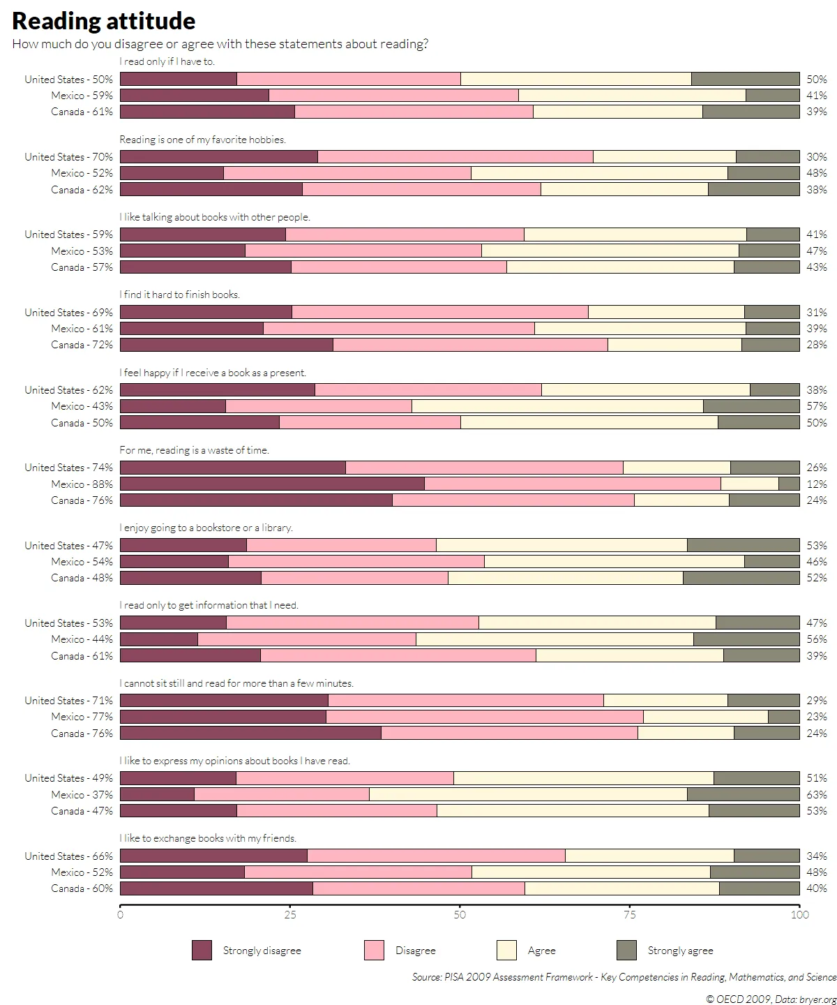
Target result
http://www.datavisualisation-r.com/pdf/barcharts_multiple_all_grouped.pdf
Long time no see.Today’s target seems weird but I would like to challenge myself to become proficient in ggplot.
#Load extra font first to avoid geom_text font error
library(extrafont)
#Load neccessary lib
library(ggplot2)
library(dplyr)
#Setting width and height. This graph has very long height

options(repr.plot.width=10, repr.plot.height=12)
theme_set(theme_minimal(base_family = "Lato Light"))
The data originate from a survey on the international comparison of school performance study by the Programme for International Student Assessment (PISA) from 2009. This survey, conducted on behest of the Organisation for Economic Co- operation and Development (OECD), recorded the abilities of 15-year-old students in the areas of reading competency, mathematical competency, and scientific competency in the OECD states and in 33 OECD partner countries. Since 2000, the survey has been conducted every 3 years.
Searching through the official website of OECD does not return any downloadable dataset.
Fortunately, someone made it as a package since 11 years ago: https://github.com/jbryer/pisa.
We take the pisa.student.rda dataset and start the work.
Note: We can dive into PISA 2018 data at here: https://www.oecd.org/pisa/data/2018database/
We tried to use readRDS function but it returns unknown input format.
Thus we use the traditional load function. However, unlike readRDS which
convert directly to a dataframe, load() does not return the object.
It produces a side effect where the objects saved in the file are loaded into the environment.
Assigning the load to a variable and we have the data loaded pisa.student and pisa.catalog.student.
#Load data
load("./myData/pisa-master/data/pisa.student.rda")
#Calling our dataframe
head(pisa.student)dim(pisa.student)475460 · 305
unique(pisa.student$COUNTRY)Because our graph only represents the data for the USA, Canada and Mexico (USMCA), we filtered it and compared the total number of respondents in the book (66,690). In addition, there are more than 300 questions but our graph extracted only the items of question group 28, i.e variables whose name starts with “ST24Q” (or 11 questions based on the targeted result image).
pisa <- pisa.student %>%
    dplyr::filter(COUNTRY %in% c('United States', 'Canada', 'Mexico')) %>%
    select(2,5, starts_with("ST24Q"))
dim(pisa)
head(pisa)
66690 · 13
load("./myData/pisa-master/data/pisa.catalog.student.rda")#Get the desc of questions
#Check type of `pisa.catalog.student`
dim(pisa.catalog.student)
is.vector(pisa.catalog.student)NULL
TRUE
#Using grep as regex searching with ^
#unname return the value of vector only
pisa.catalog.student[grep("^ST24Q", names(pisa.catalog.student))]#But the question description for our plot need to be written in a full insightful sentence
#So the above code is for the purpose of checking only
question_desc <- c("I read only if I have to.",
"Reading is one of my favorite hobbies.",
"I like talking about books with other people.",
"I find it hard to finish books.",
"I feel happy if I receive a book as a present.",
"For me, reading is a waste of time.",
"I enjoy going to a bookstore or a library.",
"I read only to get information that I need.",
"I cannot sit still and read for more than a few minutes.",
"I like to express my opinions about books I have read.",
"I like to exchange books with my friends.")
names(question_desc) <- paste0("ST24Q", sprintf("%02d", 1:11))
question_descNow we need to make our data readable by ggplot, or switch it into a longer form using pivot_longer()
library(tidyr)pisa_longer <- pisa %>%
pivot_longer(cols=c(-1,-2), names_to = "Question", values_to = "Answer") %>%
#We dropped SCHOOLID here
group_by(COUNTRY, Question, Answer, .add=T) %>%
#the default .add=FALSE in group_by() will override existing groups.
summarize(Count = n(), .groups = 'drop') %>%
#We dropped NA Answer here
filter(Answer != 'NA')
head(pisa_longer, 10)#Create percentage column
pisa_617 <- pisa_longer %>%
group_by(COUNTRY, Question, .add=T) %>%
mutate(Perc = Count / sum(Count))
head(pisa_617, 10)#The main idea is using the facet element
pisa_617 %>%
ggplot(aes(x=Perc, y=COUNTRY)) +
geom_col(mapping=aes(fill=Answer), position = position_stack(reverse = TRUE)) +
facet_grid(Question ~ .)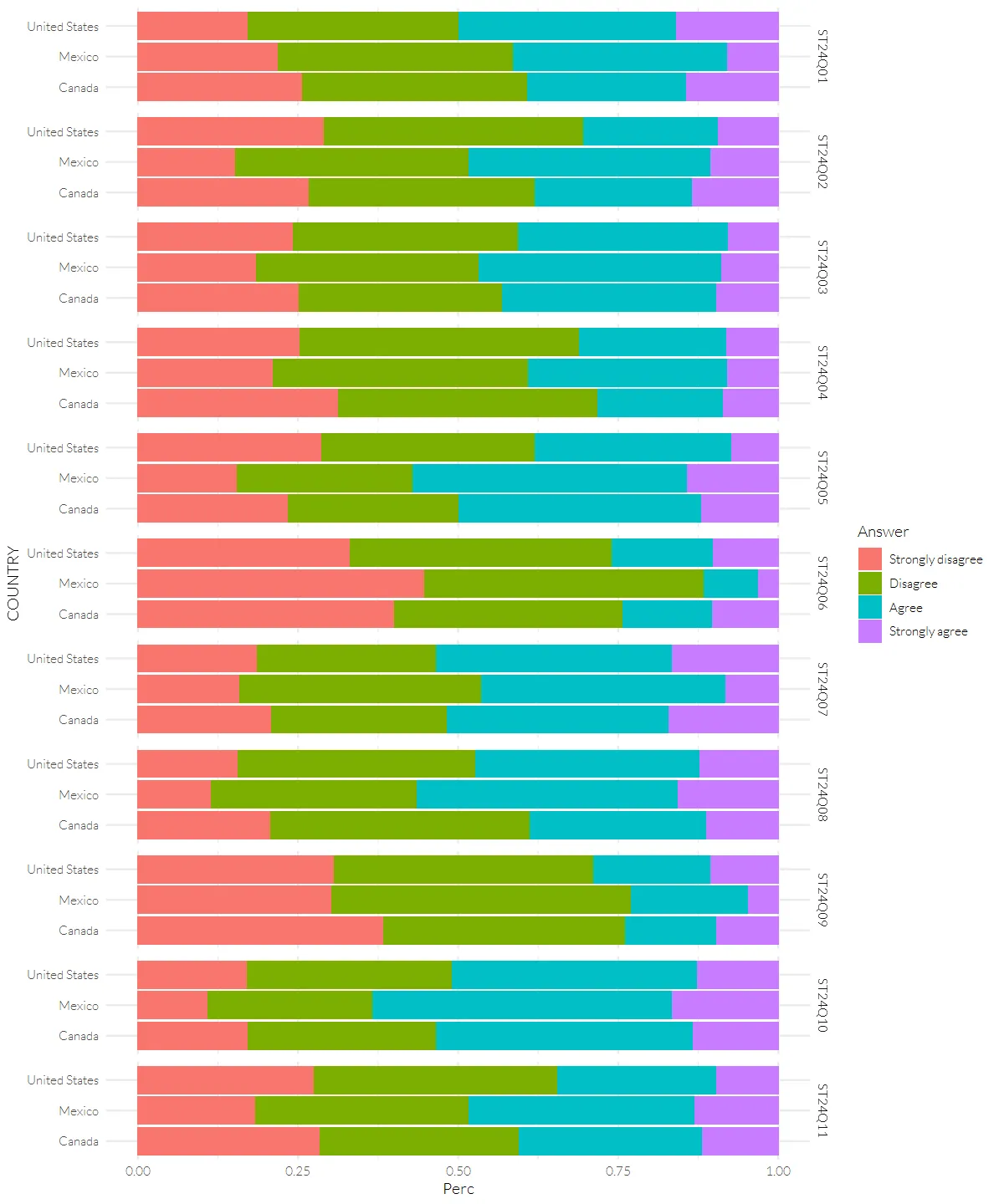
#Create custom color vector based on origin graph(using eye-dropper)
color_pisa <- c("Strongly agree" = "#8b8878",
               "Agree" = "#fff8dc",
               "Disagree" = "#ffb6c1",
               "Strongly disagree" = "#8b475d")
pisa_617 %>%
ggplot(aes(x=Perc, y=COUNTRY)) +
geom_col(mapping=aes(fill=Answer), position = position_stack(reverse = TRUE)) +
scale_fill_manual(values=color_pisa) +
scale_y_discrete(labels=function(x) paste0(x, "-")) +
facet_grid(Question ~ .)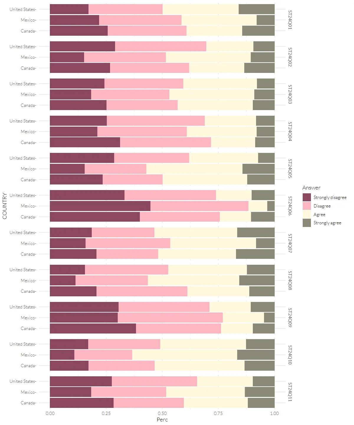
We try to edit the y - label by creating a new column.
pisa_test <- pisa_617 %>%
    group_by(COUNTRY, Question, .add=T) %>%
    mutate(neg_perc = sprintf("%.0f%%",sum(Count[Answer %in% c("Strongly disagree", "Disagree")]) / sum(Count) * 100)
          )
head(pisa_test,10)pisa_test %>%
ggplot(aes(x=Perc, y=COUNTRY)) +
geom_col(mapping=aes(fill=Answer), position = position_stack(reverse = TRUE)) +
scale_fill_manual(values=color_pisa) +
geom_text(data=pisa_test, mapping=aes(x=-0.05, y=COUNTRY, label=neg_perc), size=3, hjust=1) +
facet_grid(Question ~ .)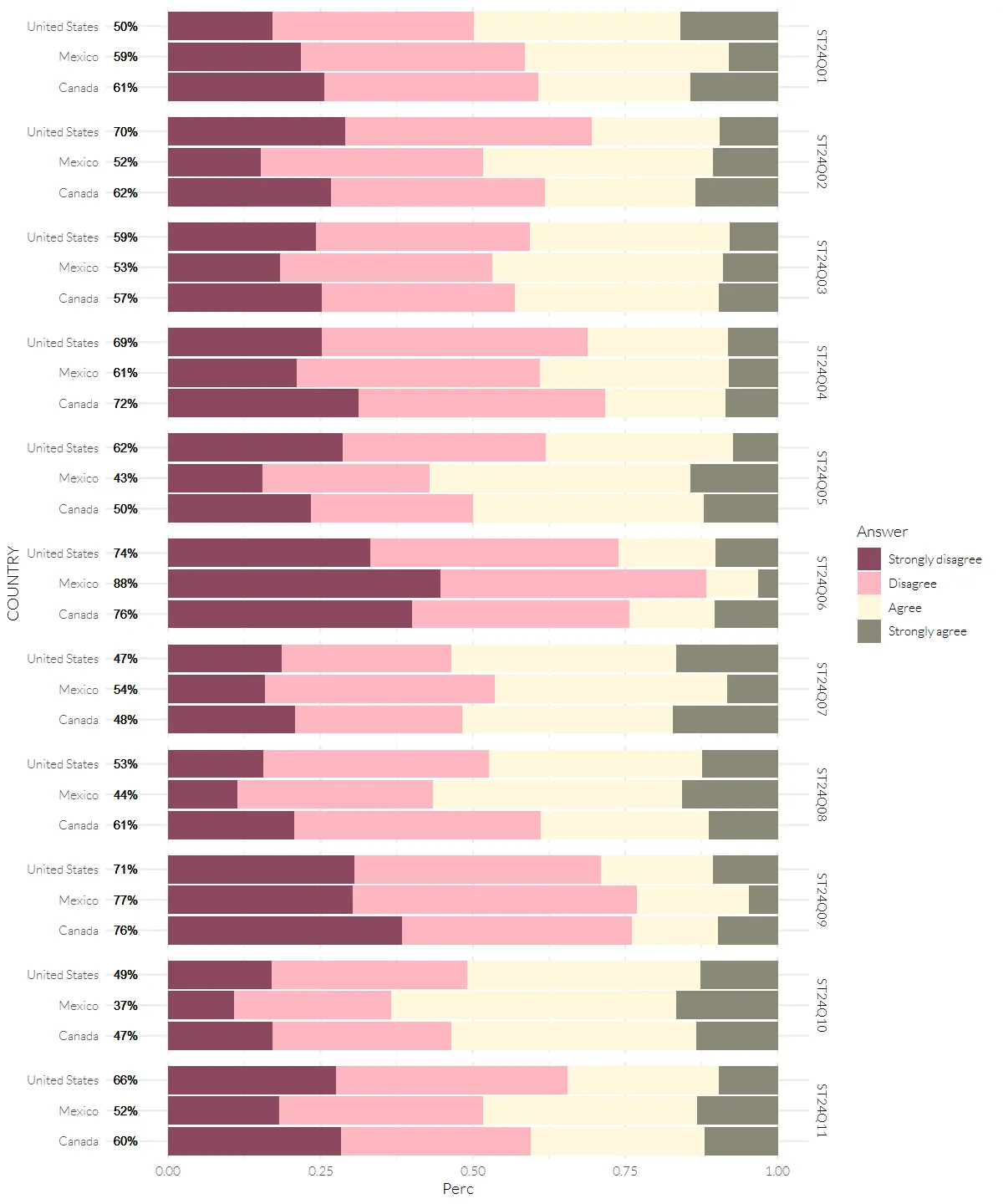
The problem arises, because the neg_perc was drawn 4 times for each country in each question. It makes the text seems bolder and aliasing. The proposed solution I found from ChatGPT is to create another column contains the desired labels (eg. Canada - 61%), but it was plotted 4 times repeatedly again.
In general, I think those are not a elegant solutions and waste of memory. So I will try to use the setting scale_y_discrete with custom function as below.
my_function <- function(breaks) {
    result <- pisa_test %>%
    group_by(COUNTRY, Question) %>%
    summarise(Percentage_Disagree = round(sum(Count[Answer %in% c("Strongly disagree", "Disagree")]) / sum(Count) * 100,0),
              .groups = 'drop')
    labels <- paste0(breaks, " - ", result$Percentage_Disagree,"%")
  return(labels)
}my_function(c('Canada', 'Mexico'))'Canada - 61%''Mexico - 62%''Canada - 57%''Mexico - 72%''Canada - 50%''Mexico - 76%''Canada - 48%''Mexico - 61%''Canada - 76%''Mexico - 47%''Canada - 60%''Mexico - 59%''Canada - 52%''Mexico - 53%''Canada - 61%''Mexico - 43%''Canada - 88%''Mexico - 54%''Canada - 44%''Mexico - 77%''Canada - 37%''Mexico - 52%''Canada - 50%''Mexico - 70%''Canada - 59%''Mexico - 69%''Canada - 62%''Mexico - 74%''Canada - 47%''Mexico - 53%''Canada - 71%''Mexico - 49%''Canada - 66%'However, the problem with breaks parameter in scale_y_discrete(labels = my_function) is:
- For each facet
Question, breaks will return a vector naming the label y -COUNTRY. And that’s all. - So for all
Question, we have the samebreaksvector, which isc('United States', 'Mexico', 'Canada') - Regardless of what we try in the custom
my_function, our function will never know what exactly theQuestionare, given the useless of Mr.breaks - As a result, we can not concatenate the specific percentage of each facet as in the targeted result.
So, I think we should move to solution using geom_text with axis.text.y = element_blank() in theme to turn of the labels of y-axis.
pisa_label <- pisa_617 %>%
    group_by(COUNTRY, Question, .add=T) %>%
    summarize(neg_perc = sum(Count[Answer %in% c("Strongly disagree", "Disagree")]) / sum(Count) * 100,
             .groups = "drop") %>%
    mutate(right_labels = sprintf("%.0f%%", 100 - neg_perc),
           left_labels = paste0(COUNTRY, " - ", sprintf("%.0f%%", neg_perc)))
head(pisa_label)p1 <-
pisa_617 %>%
ggplot(aes(x=Perc, y=COUNTRY)) +
#geom_col creates bar and customize bar color
geom_col(mapping=aes(fill=Answer), color = "black", linewidth = 0.2, width = 0.8, position = position_stack(reverse = TRUE)) +
scale_fill_manual(values=color_pisa) +
#break into facet, but use facet_wrap instead of facet_grid to modify position of strip text
facet_wrap(Question ~ ., nrow = 11, strip.position = "top",
labeller = as_labeller(question_desc)) +
#custom label, on the left and the right
geom_text(data=pisa_label, mapping=aes(x=-0.01, y=COUNTRY, label=left_labels), size=3, hjust=1, family = "Lato Light") +
geom_text(data=pisa_label, mapping=aes(x=1.01, y=COUNTRY, label=right_labels), size=3, hjust=0, family = "Lato Light") +
#Add custom axis by geom_segment
geom_segment(data=data.frame(x = 0, xend = 1, y = 0, yend = 0, Question = "ST24Q11"),
aes(x=x,y=y,yend=yend,xend=xend), inherit.aes=FALSE)+
#To move the panel area to the right, we increase the xlim while limiting the display label
coord_cartesian(xlim=c(-0.1,1), clip="off")
p1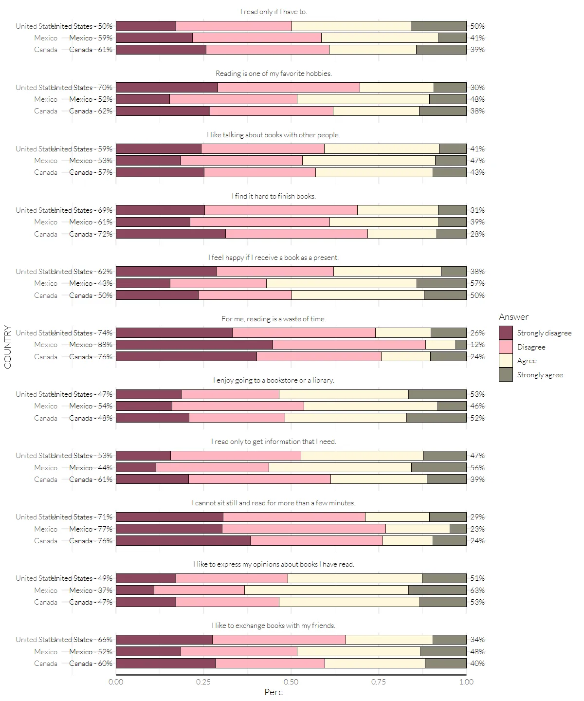
#Formating
p1  +
    #Title
    labs(x=NULL, y=NULL,
         title="Reading attitude",
         subtitle = "How much do you disagree or agree with these statements about reading?",
         caption= "Source: PISA 2009 Assessment Framework - Key Competencies in Reading, Mathematics, and Science
                    \n © OECD 2009, Data: bryer.org") +
    #Labelling x-axis
    scale_x_continuous(breaks = seq(0, 1, 0.25), labels= function(x) round(abs(x)*100,0)) +
    #Add padding between bar and x-axis
    scale_y_discrete(expand = expansion(add = .8)) +
    #Theme element
    theme(axis.text.y = element_blank(),
          panel.grid.major = element_blank(),
          panel.grid.minor = element_blank(),
          #strip text aligned with the bar.
          #Don't know the relationship btw l=30 and l=50
          strip.text.x = element_text(hjust = 0, size = 3 *14/5,
                                      margin = margin(l=90)),
          legend.position = "bottom",
          legend.title = element_blank(),
          plot.caption = element_text(face="italic"),
          plot.title.position = "plot",
          plot.title = element_text(size = 20, family="Lato Black"),
          #Add some margin to final svg output
          plot.margin = margin(t=10, l=10),
          #Show the x-axis line and ticks
          axis.ticks.x = element_line(color = "black"),
          legend.spacing.x = unit(50, "pt"),
          #Increase the distance between legend keys
          legend.text = element_text(margin = margin(l = -40)),
         )
Note: I found some useful tips in below links:
- Naming facet - labeller using another vector: https://stackoverflow.com/questions/3472980/how-to-change-facet-labels
element_text(): https://ggplot2.tidyverse.org/reference/element.html?q=margin#null- Alignment of Plot title: https://stackoverflow.com/questions/25401111/left-adjust-title-in-ggplot2-or-absolute-position-for-ggtitle
- Play with the facet axis line by using library
lemon: https://cran.r-project.org/web/packages/lemon/vignettes/facet-rep-labels.html - Add some padding around the data to ensure that they are placed some distance away from the axes: https://ggplot2.tidyverse.org/reference/scale_discrete.html
- example for using expansion vector: https://ggplot2.tidyverse.org/reference/expansion.html
- No easy way to manipulate the axis length, without external package (Apr’23): https://stackoverflow.com/questions/76091540/ggplot-axis-change-total-length, so I use geom_segment instead
- Add geom_segment to the last facet only: https://stackoverflow.com/questions/24578352/add-a-segment-only-to-one-facet-using-ggplot2. Unfortunately, we need to create a separate dataframe for the segment.
- And why size of 10 in geom_text() is different from that in theme(text=element_text()): https://stackoverflow.com/questions/25061822/ggplot-geom-text-font-size-control. The ratio is 14/5. 1 point is 1/72 inch=0.35mm, so 1 in geom_text() is 1mm, 1/0.35 =~ 14/5
- Changing the font for geom_text: https://stackoverflow.com/questions/14733732/cant-change-fonts-in-ggplot-geom-text
#As we set the option of IRKernel at 10 x 12 inches, we set the same para for ggsave
ggsave("6.1.7 Bar char Grouping all responses.svg", last_plot(), device=svg, width = 10, height = 12, units="in")
SVG image result (Open in new tab to zoom in)

TODO:
- Change geom_text to annotate for global font: The Answer is NO.
- This function adds geoms to a plot, but unlike a typical geom function, the properties of the geoms are not mapped from variables of a data frame, but are instead passed in as vectors.
- https://ggplot2.tidyverse.org/reference/annotate.html